The SQL LISTAGG function in Snowflake or Redshift (or STRING_AGG in BigQuery) are aggregation functions that condense textual data into easy-to-view reports. Similar to other aggregation functions (like SUM or MAX), these functions aggregate data according to the column names in a GROUP BY clause.
This is a common pattern for rolling up a column with a large variety of values into a column with less variety.
You might like: From Spreadsheets to SQL: Step one towards a minimum viable data stack
How LISTAGG works in SQL
Here’s an example of what it would look like in BigQuery.
Let’s say we have a table that has cities and companies, and we want to see a list of companies that are located in each city.
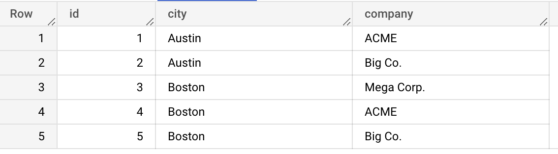
In SQL, we would write something like this:
SELECT
city,
STRING_AGG(company,', ') AS cityagg
FROM my_table
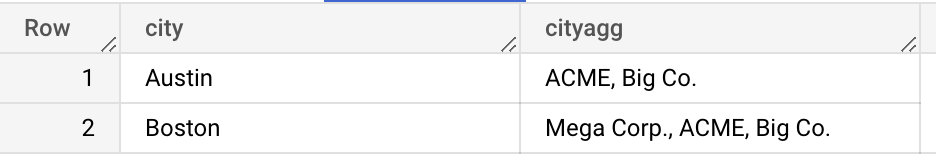
GROUP BY city;And then we would get a result that looks like this.
How to LISTAGG in Google Sheets with a Pivot Table
When I was looking for a solution to this, I found a bunch of solutions that required some pretty hairy amalgamations of the Google Sheets functions like QUERY, FILTER, and JOIN. These all felt overly complex to me because pivot tables provide the same aggregation capability that you’d find by using a GROUP BY clause in SQL.
The problem is that there is no native LISTAGG function in Google Sheets. Or so I thought!
In fact, the JOIN function does exactly what the LISTAGG function does in SQL—it just does it differently. The JOIN function takes a one-dimensional array and glues them all together with a chosen separator. This is just the same as LISTAGG, but it only works within groups.
The question is, then, how do you get the JOIN function to behave like a LISTAGG function?
It turns out to be quite simple! The answer is Calculated Fields in pivot tables.
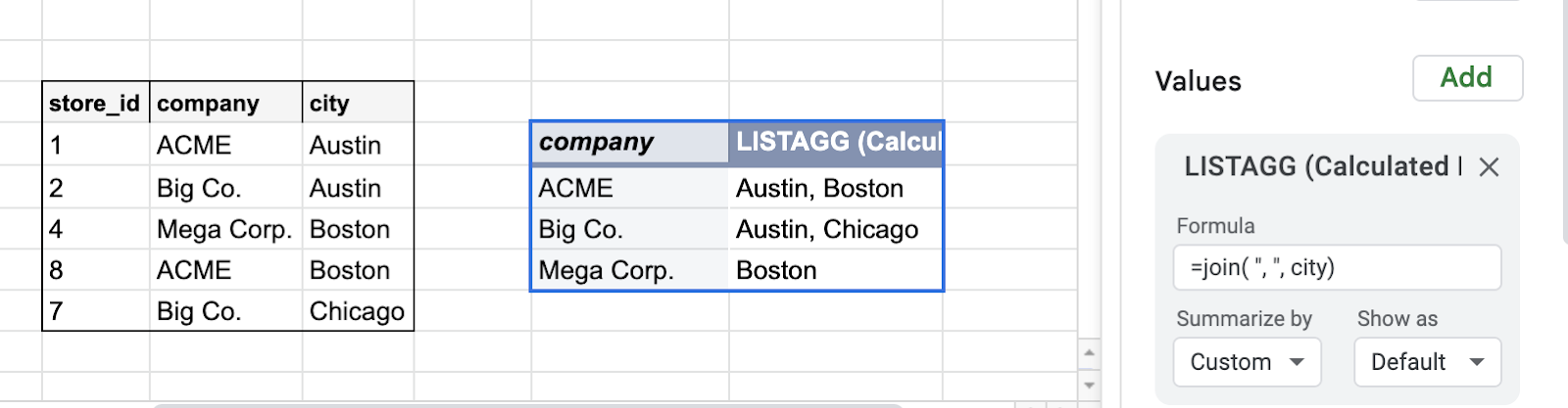
Performing a LISTAGG-like aggregation in Google Sheets is easy—just three steps:
- Create a pivot table
- Choose one or more fields to pivot into Rows
- For the aggregation Values, choose Calculated Field and use the following formula:
=JOIN(“, “, your_column_name)There are a few things to keep in mind:
- Be sure to “Summarize by” “Custom, “ or else you’ll get a value of 0 for your aggregations.
- Use lowercase column headings without spaces (or use underscores_like_this) for column names in your data. This makes it easier to set up Calculated Fields because the column reference in the Calculated Field must exactly match the column name in your data.
- Uncheck “Show Totals” because this will list all possible values in the LISTAGG’ed column. That could end up being one really long value!
That’s it! Let me know in the comments if anything is unclear. Happy aggregating!