A few days ago, Cyrus Shepard posted an example about using Levenshtein distance to compute the similarity or dissimilarity (aka the edit distance) between two strings. His example showed how to apply Levenshtein distance in Google Sheets in the context of written content, but it inspired me to demonstrate another common application: query similarity.
Since I’m teaching a course on SQL for SEO, this inspired me to demonstrate how you would calculate Levenshtein distance in BigQuery to group similar queries together and aggregate their impressions and clicks. If you want to join the course, use the promo code “CYRUS” to get $10 off!
Use the promo code “CYRUS” to get $10 off of the SQL for SEO course!
This post will provide a little background about Levenshtein distance, how to set it up in BigQuery, and walk through one simple query and spice it up into a more sophisticated query. Sign up for the course if you want to get the video walkthrough to explain the SQL!
What is Levenshtein Distance
I recommend checking out this video if you are a visual learner like me. It introduces Levenshtein distance in the context of search engines and query similarity.
The video evokes a version of search engines that were pre-Knowledge Graph and still operated in “string,” not “things.” But you can imagine a search engine today that provides predictive query completion and refinement based on Levenshtein distance…
In short, Levenshtein distance is a calculation of the number of edits to change one string of characters to another.
It’s easy to see with examples
Let’s look at the terms SEO consultant and SEO consulting. The two terms are similar (they both share “SEO consult.” That difference is found when three characters (“ant” and “ing”) are replaced. This means the Levenshtein distance is 3. Here are a few more:
| String 1 | String 2 | Operation | Levenshtein Distance |
| cat | at | 1 subtraction | 1 |
| cat | chart | 2 addition | 2 |
| cat | cats | 1 addition | 1 |
| cat | rat | 1 replacement | 1 |
| cat | cow | 2 replacements | 2 |
| cat | dog | 3 replacements | 3 |
You can see how helpful this could be in grouping similar queries.
SEO application
Tracking keyword performance is great, but if you’re dealing with a site that has a lot of long-tail, high-cardinality keywords, it’s helpful to track similar keywords together as a group. In many cases, Google will serve the same search page for long-tail queries like “xyz consultant” and “xyz consulting,” so these two queries are practically the same for Google search.
Disclaimer: It is not always the case that two similar queries are semantically the same! Google will show different results for queries that only have a Levenshtein distance of 1! You’ll see that if you look at the variation of search metrics for similar queries in Google Search Console.
Example: Go search for cat and cats.
SQL analysis
First, we have to add the Levenshtein distance calculation to BigQuery as a user-defined function since it doesn’t exist by default. Here’s a quick tutorial on that, but it’s as simple as running this CREATE FUNCTION command. This will add this function to the schema that houses your Google Search Console data in BigQuery.
CREATE OR REPLACE FUNCTION searchconsole.levenshtein(x STRING, y STRING)

RETURNS INT64

LANGUAGE js

AS r"""

   const track = Array(y.length + 1).fill(null).map(() => Array(x.length + 1).fill(null));

  for (let i = 0; i <= x.length; i += 1) {
     track[0][i] = i;
  }

  for (let j = 0; j <= y.length; j += 1) {
     track[j][0] = j;
  }

  for (let j = 1; j <= y.length; j += 1) {
     for (let i = 1; i <= x.length; i += 1) {
        const indicator = x[i - 1] === y[j - 1] ? 0 : 1;
        track[j][i] = Math.min(
           track[j][i - 1] + 1, // deletion
           track[j - 1][i] + 1, // insertion
           track[j - 1][i - 1] + indicator, // substitution
        );
     }
  }

  return track[y.length][x.length];

""";
Calculating Levenshtein Distance in SQL
Now, we can run this query to start applying the calculation to our Google Search Console data in Bigquery.
SQL query
WITH queries AS (
 SELECT query,
   SUM(impressions) AS impressions,
   SUM(clicks) AS clicks
 FROM `<project-name>.searchconsole.searchdata_site_impression`
 WHERE data_date > CURRENT_DATE() - 7
   AND query IS NOT NULL
 GROUP BY query
),

query_combinations AS (
 SELECT
   q1.query AS main_query,
   q2.query AS sub_query,
   q1.clicks AS main_clicks,
   q2.clicks AS sub_clicks,
   q1.impressions AS main_impressions,
   q2.impressions AS sub_impressions,
   searchconsole.levenshtein(q1.query, q2.query) AS levenshtein_distance,
   row_number() over (partition by q2.query order by q1.impressions desc) rn
 FROM queries q1
 CROSS JOIN queries q2
 WHERE q1.query <> q2.query
   AND q1.impressions > q2.impressions
   AND searchconsole.levenshtein(q1.query, q2.query) < ceil(length(q1.query) / 4) -- Threshold for grouping subordinate queries
)

select * from query_combinations
Explanation
This query has two parts. The first part is the `queries` common table expression (CTE) that aggregates the total number of impressions and clicks for each unique search query from the searchdata_site_impression table over the last 7 days. This step ensures that only non-null queries are considered and summarizes each query’s search performance metrics. Note: Filtering data during this step is really important!
The second CTE, query_combinations, generates all possible combinations of the queries using a cross-join and calculates the Levenshtein distance between them to determine their similarity. For each pair of queries, it identifies a “main query” (the one with more impressions) and a “subordinate query.” The ROW_NUMBER() function is used to assign a ranking to each subordinate query within its group based on the impressions of the main query. The filtering condition ensures that only pairs with a similarity threshold (as determined by the Levenshtein distance) are included.

Now, you can see the Levenshtein distance (similarity) between queries in your data. Note that the row number calculation will be used in the next query.
Grouping and aggregating similar queries
Now, let’s get into something you just can’t do in spreadsheets! Let’s group queries together so we can roll up the metrics for similar subordinate queries into more common main queries. Here’s the complete query.
SQL query
WITH queries AS (
SELECT query,
SUM(impressions) AS impressions,
SUM(clicks) AS clicks
FROM `mvp-data-321618.searchconsole.searchdata_site_impression`
WHERE data_date > CURRENT_DATE() - 7
AND query IS NOT NULL
and query like '%consult%'
GROUP BY query
),
query_combinations AS (
SELECT
q1.query AS main_query,
q2.query AS sub_query,
q1.clicks AS main_clicks,
q2.clicks AS sub_clicks,
q1.impressions AS main_impressions,
q2.impressions AS sub_impressions,
searchconsole.levenshtein(q1.query, q2.query) AS levenshtein_distance,
row_number() over (partition by q2.query order by q1.impressions desc) rn
FROM queries q1
CROSS JOIN queries q2
WHERE q1.query <> q2.query
AND q1.impressions > q2.impressions
AND searchconsole.levenshtein(q1.query, q2.query) < ceil(length(q1.query) / 4) -- Threshold for grouping subordinate queries
),
grouped_queries AS (
SELECT
main_query,
ARRAY_AGG(
STRUCT(
sub_query,
sub_clicks,
sub_impressions,
levenshtein_distance
)
) AS subordinate_query_stats,
SUM(sub_clicks) AS total_sub_clicks,
SUM(sub_impressions) AS total_sub_impressions,
MAX(main_clicks) AS main_clicks, -- Ensure the main query's clicks are retained
MAX(main_impressions) AS main_impressions -- Ensure the main query's impressions are retained
FROM query_combinations
WHERE rn = 1
GROUP BY main_query
)
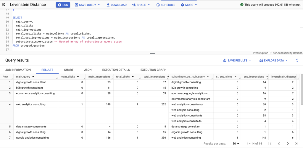
SELECT
main_query,
main_clicks,
main_impressions,
total_sub_clicks + main_clicks AS total_clicks,
total_sub_impressions + main_impressions AS total_impressions,
subordinate_query_stats -- Nested array of subordinate query stats
FROM grouped_queries;
Explanation
Continuing from the previous explanation, the query further processes the results to group similar search queries under a “main query” using a third Common Table Expression (CTE) called grouped_queries. This CTE aggregates the subordinate queries for each main query that passed the similarity threshold defined in the query_combinations CTE. It uses ARRAY_AGG to compile a nested array of subordinate query statistics, which includes the subordinate query text, its click and impression counts, and the Levenshtein distance to the main query.
Additionally, the grouped_queries CTE calculates the total clicks and impressions for all subordinate queries associated with each main query. It also retains the main query’s own click and impression counts using the MAX function. The condition WHERE rn = 1 ensures that only the most relevant (highest impressions) subordinate query for each unique main query is included in the final grouping.

The final SELECT statement produces the output that presents each main query along with its total clicks and impressions, which are calculated by adding the main query’s metrics to the aggregated subordinate query metrics. It also provides a nested structure (subordinate_query_stats) that contains detailed statistics for each subordinate query. This comprehensive output enables deeper analysis of the relationship and performance of similar search queries, helping to identify trends and optimize search strategy around the most effective queries.
Feeling inspired?
If this seems powerful to you (because it is!), you should sign up for my SQL for SEO course! It covers more than just SQL. It also demystifies all the foundational knowledge that you’ll need to get up and running with BigQuery for SEO analytics.
Since you read this far, you can use the promo code “CYRUS” to get $10 off the premium course!