Dynamic Gantt Charts in Google Sheets + Project Timeline Template
August 17, 2018
Google Docs and Gantt charts are a perfect match. Google Spreadsheets offers the ability to share and update spreadsheets in real-time, which is a major benefit for any project team, especially those who work in different locations or time zones. On top of that, you can’t beat the free price!
Many projects are complex enough to demand a formal task planning and management hub but do not justify a full-featured, premium application. This tutorial will show you how to take your ordinary task list and turn it into a dynamic visual timeline—a Google Spreadsheet Gantt chart.
View the Sample Chart with Formatting Examples
View a Comprehensive Template From a Reader
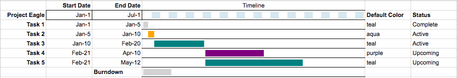
There are other Google Spreadsheet Gantt chart examples that use the Chart feature as the visualization. I like to use the SPARKLINE() function. This keeps the project task visualization in the same place as all the important details about each task such as the RACI assignments or progress updates.
Dynamic Sparklines Work Better Than Charts
Sparklines are essentially just little data visualizations in spreadsheet cells. To learn more about how the sparkline feature works, check out these sparkline examples. To create the visualization, we will use “bar” for the value of “charttype.” Then we get a little bit clever with colors to show each task’s start and end dates. The SPARKLINE formula for each task visual looks like this:
=SPARKLINE({INT(taskStart)-INT(projectStart), INT(taskFinish)-INT(projectFinish)},{"charttype","bar";"color1","white";"empty","zero"; "max",INT(projectFinish)-INT(projectStart)})
The projectStart and projectFinish values are the start and end date of the project, and the taskStart, and taskFinish values are the start and end dates for the task that is being shown in the timeline visualization.
The reason everything is being wrapped in the INT() function is so that the dates can be subtracted from each other to provide the difference in days. The first argument to SPARKLINE puts two values in the array literal that are essentially:
{daysSinceProjectStartUntilTaskStart, daysSinceProjectStartUntilTaskFinish}
The SPARKLINE function then makes two bars, one which is colored "white", as to be invisible and the other which is colored blue (by default) or any color you choose by setting "color2". The value for "max" is the difference between the start and end of the project in days.
On the example template, there are a couple other features: a week-by-week ruler and the burndown visualization.
The week-by-week visualization uses a clever little formula to make an array of number incrementing by seven as the first argument to SPARKLINE to display alternating colored bars for each week of the project’s duration.
split(rept("7,",round((int(projectEnd)-int(projectStart))/7)),",")
The burn down visualization shows the days that have been burned through the project. This gives you a visual display of how well the project is keeping on track to its timeline. The first argument to SPARKLINE is a dynamic value, calculated by subtracting the project’s start date from the current date:
int(today())-int(projectStart)
Customizing your Timelines
Each SPARKLINE function takes arguments for color1 and color2. These values set the color of the alternating bars in the bar visualization. For each task, color1 is set to white so to be invisible. But color2 can be set to anything that may be useful for managing your project. Colors could be specified by task owner or type, or even by dynamically set based on if they are ahead of schedule, in progress, late, etc…
Keep this in your Google Docs project folder with all of your other important project documentation for a neat project hub.
Simplifying Your Spreadsheet Formulas
The SPARKLINE functions, especially if you use a lot of conditional coloring, have a tendency to become really long and hard to maintain. To make it easier to update and maintain, I suggest using named ranges. Named ranges allow you to designate a few cells that hold color variables that you can refer to by name.
For example, if you wanted all the future tasks to be the color blue then in cell C2, you could input the text “blue.” Then you could name that cell futureColor and everytime you needed to reference the “future color,” use futureColor in the formula. Then you don’t have to think about cell references and you only have to update one cell to update several sparklines. This also works for project start and end dates and fixed miles stones. It does not work for variable dates like task start and end dates, those should be cell references.